Logistic Regression and Counterfactual Thinking with Titanic Survivorship Data

This project uses data on the passengers of the Titanic to create a logistic regression that predicts the probability that a given passenger survived the disaster. The accuracy of this model is evaluated via a proprietary system of accuracy measurement for these types of discrete probability predictions from the author’s prior work. This logistic model is then used to answer counterfactual questions about changes in the probability of survival based on passenger class and sex.

Data and Problem Statement

The RMS Titanic was a famous passenger ship that sunk in the North Atlantic ocean on April 15, 1912. Approximately 38% of passengers survived the disaster.

But is there a way to tell who had the best probability of survivorship?

What known factors influenced whether a passenger survived or not. What if, for a given passenger, the personal factors contributing to his or her survival had been different?

This project creates a logistic regression model to predict each Titanic passenger’s probability of survival based on various predictor variables. To accomplish this, a Titanic Dataset uploaded by M Yasser H on Kaggle is used. [1] This dataset provides information on 891 Titanic passengers, whether or not they survived the disaster, and other pertinent data such as the passenger class, sex, age, etc. for each such passenger.

After the model is established, it is used to think counterfactually about how hypothetical changes to certain predictors (i.e. passenger class and sex) would impact a passenger’s probability of survival and what influence those predictors have on such probability, overall.

Looking at Survivorship Aboard the Titanic

There are 891 passengers listed in the dataset. For each passenger, the dataset presents a Survived variable which is coded as either 1 (i.e., the passenger survived) or 0 (i.e. the passenger did not survive).

There were many more casualties than passengers that survived.

FIGURE 1. Distribution of Survivorship of Passengers Abord the RMS Titanic.

It would be well and good, and certainly done before [2] to plot the number of survivors based on passenger class, age, sex, etc. in the form of boxplots like Figure 1. This would give us the overall picture of who survived and who didn’t.

But what we’re really after in this project is to ask and answer questions like: “What if Passenger X had been male instead of female?” or “What is Passenger Y had been in First Class instead of Third Class?”

In order to answer these counterfactual questions (i.e., questions counter to the real facts), we first must build a model that tells us the probability of a given passenger surviving the Titanic’s sinking with the information known.

To this, we turn first.

Major Steps in This Project

This project involves the following major steps:

1. Choose Predictors
2. Establish Priors
3. Form the Predictive Model
4. Check the Model’s Accuracy
5. Apply Counterfactual Thinking

The R code used for this project is available in the References section at the end of this project page. [3]

Establishing Priors

Two normal priors were set on the intercept and ß (that is, response) variables:

• Intercept ~ 𝒩(logit(0.38), 1.5)
• ß ~ 𝒩(0, 1)

The prior on the intercept was chosen because approximately 38% of passengers survived the disaster. This is known. The prior on the predictors is weakly informative with a mean of 0.

Choosing Predictors

When choosing predictors, the dataset provides seven to choose from:

1. PClass = passenger class
2. Sex = passenger sex
3. Age = passenger age
4. SibSp = passenger’s number of siblings or spouses aboard
5. Parch = passenger’s number of parents or children aboard
6. Fare = cost of passenger’s fare
7. Embarked = the port where the passenger boarded the ship

Looking at Figure 2, we see only clear correlations between Pclass, Sex, and Age with the response variable, Survived.

FIGURE 2. Correlation of Survivorship and Available Predictors

Thus, only those three predictors were chosen for the model.

Several tests were run with a varying combination of predictors, including the use of intersectional predictors (such as Pclass * Age, Sex * Age, Pclass * Sex, etc.). The model presented here preformed reliably well when compared to more complex models. For the sake of simplicity and ease of calculation, only these three predictors were used.

Forming the Predictive Model

According to our chosen predictors, our model takes the form:

P(Survived) ~ Pclass + Sex + Age

Running the model in the R package brms [4] gives the following summary:

TABLE 1. Summary of the Logistic Regression Model from the brms Package in R.

Family: bernoulli 
Links: mu = logit 
Formula: Survived ~ Pclass_z + Sex_z + Age_z 
Data: data (Number of observations: 891) 
Draws: 4 chains, each with iter = 2000; warmup = 1000; thin = 1;
       total post-warmup draws = 4000

Regression Coefficients:
           Estimate Est.Error l-95% CI u-95% CI Rhat Bulk_ESS Tail_ESS
Intercept      1.35      0.15     1.07     1.65 1.00     4453     3113
Pclass_z.L     1.59      0.17     1.26     1.93 1.00     4014     3349
Pclass_z.Q    -0.04      0.17    -0.36     0.29 1.00     5022     3131
Sex_zmale     -2.53      0.18    -2.89    -2.19 1.00     4460     3124
Age_z         -0.42      0.09    -0.61    -0.24 1.00     3894     3336

Taking a look at the posterior predictive check of the model, we find Figure 3.

FIGURE 3. Posterior Predictive Check of the Logistic Regression Model (100 Draws).

Our model seems to fit the data quite well. As shown in Figure 4, we can see the actual Survived (0 or 1 only) with the predicted probability of survival for each of the 891 passengers.

FIGURE 4. Actual vs. Predicted Survival Probability.

How accurate is our model at predicting real outcomes? We move next to answer this question.

Checking the Model’s Accuracy

This author has written previously on verifying the accuracy of these types of discrete probability models [5].

In that previous work, three main accuracy metrics are given. Table 2 provides us with a brief summary of these.

TABLE 2. Brief Definition of Accuracy Metrics.

Term	Definition
Â	Prediction accuracy. This is a measure of how accurate a predictor’s predictions have been.
Â’	Posterior prediction accuracy beta distribution. This is a beta distribution describing the posterior probability of a predictor’s prediction accuracy, formed by a prior based on a discrete uniform probability distribution (DUPD) and a binomial likelihood based on the predictor’s observed prediction accuracy.
P(Â’) > DUPD	Probability that a predictor’s prediction accuracy beats the DUPD; e.g., if there are two possible outcomes from a contest, the DUPD is 0.5000 (that is, a 50% probability of either outcome); P(Â’) > DUPD thus finds the probability that a predictor can beat an accuracy of 0.5000.

Let us determine these for our model, each in turn.

Â

To calculate Â, we sum the “credit” earned by our model’s predictions.

The credit earned is the probably assigned by the model to the correct outcome. For instance, for Observation 1 the model predicted a probability of 0.1127 for survival, which implies a probability of 0.8873 for not surviving. Observation 1 did not survive, so the model gains credit of 0.8873 for that observation (in essence: the model was 88.73% “correct” for that observation).

The total “credit” earned by the model was 630.6172.

This is divided by the total number of predictions made, in our case, the total number of observations (891). This is because each prediction is “worth” a value of 1 (the maximum extent of the probability space for each individual prediction). And our “credit” for each prediction is the portion of which the model guessed correctly.

Thus  is:

Our model is 70.78% accurate.

The  metric in this case does not need to be “time-weighted,” as described in prior work [5], since all predictions are made post hoc.

Â’

With  established, we turn now to form our posterior beta distribution, ’, that will help us determine the probability that our model exhibits real skill in predicting outcomes.

The following is a very brief summary of how this was done, pursuant prior art [5]:

Prior

There are 891 observations in our dataset. The prior is based on a discrete uniform probability distribution (DUPD), which assumes that an equal probability of each possible outcome.

Since we have binary outcomes—survival is either 0 (“no”) or 1 (“yes”)—the prior assumes each outcome would be correct half the time and incorrect half the time.

Thus, the prior distribution is a beta distribution with the following parameters:

α = 445.5

ß = 445.5

π = Beta(445.5, 445.5)

Likelihood

The likelihood distribution is the the number of “successes” (s) and the number of “failures” (f) from our model. The “successes” is the summed “credit” achieved by our model’s predictions, and the “failures” are the total number of predictions made, minus the “successes”. This is essentially Â.

Thus, the likelihood distribution is a binomial distribution with the following parameters:

s = 630.6172

f = 260.3828

ℓ = Binomial(630.6172, 260.3828)

Posterior

The posterior distribution will be a beta distribution that conforms to the following:

In this case, that is:

p = Beta(α+s, ß+f)

We are left with a posterior beta distribution of Beta(1,076.1172, 705.8828). This is Â’.

P(Â’) > DUPD

We can now use our posterior distribution of Beta(1,076.1172, 705.8828) to find out the probability that Â’ beats the assumptions made by the DUPD. In other words, we want to know the probability that our model’s predictions beats guessing the outcome, or the probability that its outcomes are >0.5000 (since we have a binary outcome).

The P(A’) > 0.5000 is 1. There is certainty that our model performs better that guessing. Figure 5 illustrates the case. The entire posterior distribution is well above P(x) = 0.5000.

FIGURE 5. Probability That Â’ Beats the DUPD.

As we can see from these measurements of accuracy, our model performs well for us. Now, let’s see what our model tells us about the survivability of different passenger types.

Counterfactual Thinking

We might be left wondering what the probable impact of these differences in passenger type are and how we can determine them.

For instance, it is well known that passengers in first and second class had a much higher survivability than those in third class and that females had a much higher survivability than males.

But by how much?

It would be tempting, once again, to compute simple averages and plot a few nice bar graphs showing us this. But this is the wrong way to think about these kinds of questions. This is simply because passengers are not all the same. Not all passengers in first class were the same sex or the same age, for instance. And not all female passengers were in the same class or were of the same age, etc.

What we want is to control for just one variable at a time, the variable of interest, and see what changing that variable for everyone does for their survivability.

This is counterfactual thinking: “What would it have been like if X was Y instead?”

We do this first for passenger class, then for sex, and finally, we apply this kind of thinking to four handpicked passengers to illustrate the impact of survival probability at the individual level.

The work in this section is rooted in the excellent work of Pearl, Glymour, and Jewell [6], which is an introduction to the deeper and prior work of Pearl on the subject [7].

The Concept of “Interventions” and Do Calculus

In counterfactual thinking, an “intervention” is the action of changing a variable in a model to some other variable and seeing what the outcome is. For instance, if Passenger X was in second class, male, and 41 years old, an intervention would be made by changing his age to 30, calculating the new probability of his survival, and then making a comparison. What this accomplishes is understanding what a change in age does for this one passenger, given all other established considerations.

This hinges on the simple notion of “do calculus” [6] [7].

“Do calculus” uses special notation, like P(Survived) | Age(do=30), which means the “probability of survival given that we’ve actioned age to 30,” to note the interventions made.

We will make some use of this notation, but the discussion that follows is largely free of mathematical notation and focuses on the logic of these interventions and what they tell us. Calculations can be seen in the accompanying R code [3].

Let us now turn to performing interventions on the predictor variables Pclass and Sex before we perform interventions on a few handpicked individuals.

Survivability by PClass

It is well known that passengers in the first and second classes experienced much greater rates of survival than did those in third class.

To find out the counterfactual effects of class changes, the following steps were performed for each of six possible changes in class:

1. Create a data frame for each Pclass: 1, 2, and 3. These three data frames contain only passengers of that class.
2. Create mutated data frames where each Pclass is changed to another Pclass (for instance, a change from Pclass 3 to Pclass 1, etc.). This leaves us with 6 such mutated data frames. These are our interventions.
   • Pclass 1 -> 3
   • Pclass 1 -> 2
   • Pclass 2 -> 1
   • Pclass 2 -> 3
   • Pclass 3 -> 1
   • Pclass 3 -> 2
3. Predict the Survived probability for each of the six mutated Pclasses. This are our counterfactuals. These 6 sets of predictions now tell us what would have been had passengers’ Pclass been altered.
4. Compare each of the mutated data frames mean Survived probability with that of the newly predicted counterfactual Survived probabilities. This leaves us with the mean difference due to our interventions.

The results of these interventions are shown in Figure 6 and summarized in Table 3.

FIGURE 6. Changes in Predicted Probability of Survival Based on Changes in Class.

TABLE 3. Changes in Class and Effects on Probability of Survival on the Titanic
Change	Probability
3 to 2	+0.1791
3 to 1	+0.3821
2 to 3	−0.1867
2 to 1	+0.1856
1 to 2	−0.1779
1 to 3	−0.3582

Indeed, changes in lower class to higher class had positive effects on Survived probability, and vice versa.

Survivability by Sex

The same types of interventions were performed for the variable Sex. The mean predicted Survived probability for each passenger Sex was compared to the mean predicted Survived probability of the intervened (that is changed) passenger Sex.

The results are visible in Figure 7 and summarized in Table 4.

FIGURE 7. Changes in Predicted Probability of Survival Based on Changes in Sex.

TABLE 4. Changes in Sex and Effects on Probability of Survival on the Titanic
Change	Probability
Female to Male	−0.4871
Male to Female	+0.4827

Keeping all other variables constant, had the mean female passenger been male instead, that passenger’s mean Survived probability would drop by 0.4871. The reverse scenario would increase the passenger’s mean Survived probability by 0.4827.

These two interventions—Pclass and Sex—are interesting and useful in determining the impact of the predictors on the response.

But what is more interesting and useful still is performing interventions on individuals.

The Survivability of Four Individuals

Four individuals (IDs 1, 4, 21, and 53) were chosen from the dataset. These four were chosen as a fairly diverse group of people with different PClass, Sex, and Age variables, and consequently, different predicted Survived probabilities from our model. These four individuals are shown in Table 5.

TABLE 5. Actual Variables of Four Selected Passengers.
ID	Name	Survived	Pclass	Sex	Age	Prediction
1	Braund, Mr. Owen Harris	0	3	male	22	0.1127
4	Futrelle, Mrs. Jacques Heath (Lily May Peel)	1	1	female	35	0.9062
21	Fynney, Mr. Joseph J	0	2	male	35	0.2123
53	Harper, Mrs. Henry Sleeper (Myna Haxtun)	1	1	female	49	0.8603

For these four individuals, we wish to perform four interventions, similar to those we performed on the various Pclass groups and Sex groups.

The following interventions were performed:

• ID 1: P(Survived) | Pclass([do=1]) + Sex(male) + Age(22)
• ID 4: P(Survived) | Pclass(1) + Sex([do=male]) + Age(35)
• ID 21: P(Survived) | PClass([do=1]) + Sex([do=female]) + Age(35)
• ID 53: P(Survived) | PClass([do=3]) + Sex(female) + Age([do=29])

That is:

• For ID 1 we change Pclass from 3 -> 1.
• For ID 4 we change Sex from female -> male.
• For ID 21 we change Pclass from 2 -> 1 and Sex from male -> 1.
• And for ID 53 we change Pclass from 1 -> 3 and Age from 49 -> 29.

The new variables for these four individuals are shown in Table 6.

TABLE 6. Counterfactual Variables of Four Selected Passengers.
ID	Name	Survived	Pclass	Sex	Age	Prediction
1	Braund, Mr. Owen Harris	0	1	male	22	0.1127
4	Futrelle, Mrs. Jacques Heath (Lily May Peel)	1	1	male	35	0.9062
21	Fynney, Mr. Joseph J	0	1	female	35	0.2123
53	Harper, Mrs. Henry Sleeper (Myna Haxtun)	1	3	female	29	0.8603

We use our model to predict the new counterfactual Survived probabilities to illustrate how these interventions impact them. The summaries are shown in Table 7.

TABLE 7. Original and Counterfactual Survival Probabilities.
ID	Name	Original	Counterfactual
1	Braund, Mr. Owen Harris	0.1127	0.6068
4	Futrelle, Mrs. Jacques Heath (Lily May Peel)	0.9062	0.3987
21	Fynney, Mr. Joseph J	0.2123	0.8950
53	Harper, Mrs. Henry Sleeper (Myna Haxtun)	0.8603	0.5780

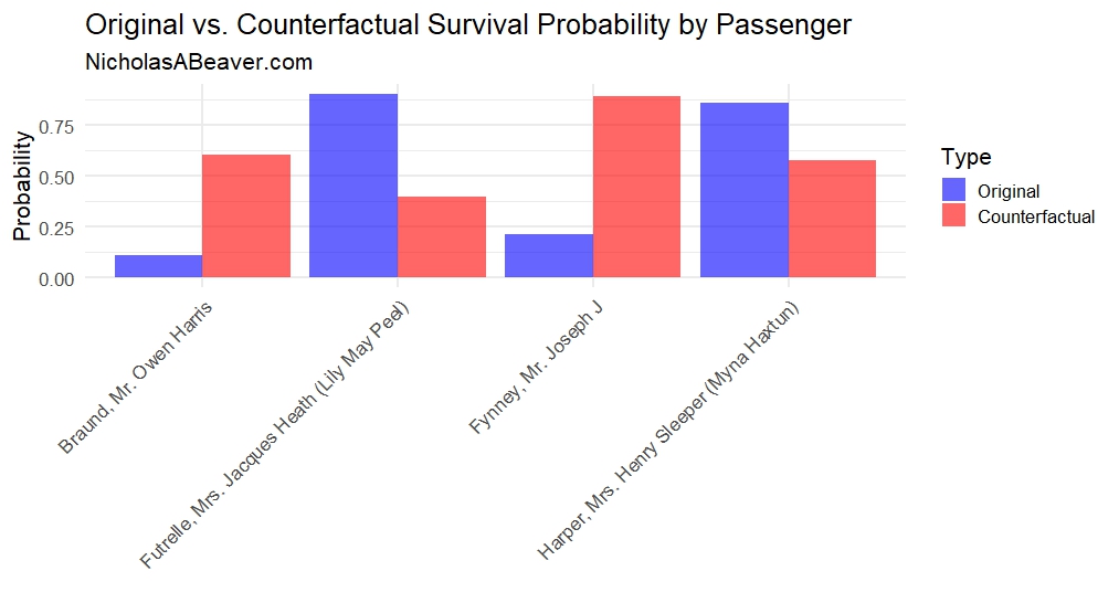
It’s very clear that, according to our previous analysis, Pclass and Sex have a strong influence on Survived probability. We can demonstrate this at the level of the individual. Figure 8 further illustrates these changes.

FIGURE 8. Original vs. Counterfactual Survival Probability by Passenger.

Conclusions

This project modeled the probability of survival on the Titanic for all 891 documented passengers. This took the form of a logistic regression model which used survival (a binary outcome) as its response and passenger class, passenger sex, and passenger age as its predictors.

The model demonstrated sufficient accuracy measured by both  (~0.7078) and P(’) > DUPD, that is, the probability that the model exhibited real predictive skill (which came to be 1, or 100%).

With confidence in the model, we computed counterfactuals to illustrate the impact of passenger class and passenger sex on survivability. This counterfactual reasoning was then applied to several handpicked individual passengers to further illustrate these impacts.

Survival during the Titanic disaster was largely a function of being in first class and female as the most impactful predictors analyzed. It should be noted, too, that while not discussed here, as shown on Table 1, the regression coefficients demonstrate that passenger age has an inverse correlation with survival (meaning that younger passengers had a higher probability of survival than did younger ones). For the sake of brevity, we did not delve into Age in this project, but the methods established here can be used to model the impact Age would have on Survived probability.

Further Work

In working on this project, the author thought about the error between the actual survival of each individual passenger (that is: either 0 or 1) and the predicted probability that that individual passenger survive.

These errors are due to the model’s inability to account for other, outside, variables. These influential factors are unknown.

Figure 9 plots each passenger’s computed error.

FIGURE 9. Error Between Actual and Predicted Survival Probability.

Future work may involve using these errors to compute a sort of “personal survivability modifier” that helps account for the individual circumstances faced by passengers that influenced their outcomes.

For instance, if Passenger Z survived, thus his or her variable Survived = 1, and our model computes a survival probability of 0.72, Passenger Z’s error is -0.28 (that is, the model underpredicts the true outcome by 0.28). When we think counterfactually about this passenger—”what if Passenger Z was in class A instead”—this “personal survivability modifier—might “follow” Passenger Z from what actually occurred into the counterfactual universe in some way. In other words, because Passenger Z exhibited a higher outcome that his or her computed survival probability, this error (in this case, in the positive direction) should be made to influence any counterfactual probabilities as a proxy for other unknown factors that contributed to Passenger Z’s survival.

Food for thought.

References

1. Yasser H (2021). Titanic Dataset: Titanic Survival Prediction Dataset [.csv file]. Kaggle.com. https://www.kaggle.com/datasets/yasserh/titanic-dataset
2. Abdel-Hamid, T.M. (2024). Classification PRJ – Classify Survived or not. Kaggle.com. https://www.kaggle.com/code/tarekmuhammed/classification-prj-classify-survived-or-not
3. Beaver, N.A. (2025). R Code for Logistic Regression and Counterfactual Thinking with Titanic Survivorship Data [.txt file]. Published 3 July 2025. NicholasABeaver.com. https://www.nicholasabeaver.com/wp-content/uploads/2025/07/R_code_for_logistic_regression_and_counterfactual_thinking_with_titanic_survivorship_data.txt
4. Bürkner, P.C. (2017). brms: An R package for Bayesian multilevel models using Stan. Journal of Statistical Software, 80(1), 1–28. https://doi.org/10.18637/jss.v080.i01
5. Beaver, N.A. (2025). An Accuracy Rating System for Discrete Probability Predictions Using Sportsbook Odds for Super Bowl LIX. Published 23 June 2025. NicholasABeaver.com. https://www.nicholasabeaver.com/portfolio/an-accuracy-rating-system-for-discrete-probability-predictions-using-sportsbook-odds-for-super-bowl-lix/
6. Pearl, J., Glymour, M., and Jewell, N.P. (2016). “Causal Inference In Statistics: A Primer”. John Wiley & Sons.
7. Pearl, J. (2009). “Causality: Models, Reasoning, and Inference (Second Edition)”. Cambridge University Press.