Sales Forecasting with Eight Different Methods: Is Simpler Better?

Introduction

Sales and revenue forecasting is an essential analytical function in all types of businesses and organizations. Methods for forecasting range from simple to complex.

While all forecasting methods and their intricacies are beyond the scope of this post, I thought it would be interesting to compare eight commonly used forecasting methods side-by-side.

Organized, roughly, from simplest to most complex they are:

1. Moving average (MA)
2. The averages of the same previous calendar months (“Previous Averages”)
3. The averages of the same previous calendar month and the previous month (“Previous Period + Month”)
4. Exponential Smoothing
5. Excel’s Forecast Sheet tool
6. Seasonal Autoregressive Integrated Moving Average (SARIMA)
7. Meta’s Prophet
8. A random forest machine learning model (ML)

I explain these eight methods in a bit more detail later in this post.

The results of each of these methods are measured by the following metrics:

• R² (R-squared)
• RMSE (root mean squared error)
• sRMSE (scaled root mean squared error)
• TAE (what I call “total absolute error,” a percentage measure of how much the total predicted values vary, in absolute terms, from the actual values

After the results are determined a discussion about which methods work best and why is given along with concluding remarks.

I admit, openly, that is is very much a toy experiment. The dataset is far from complete and the methods employed are more a “quick and dirty” sort of iteration. But I hope to illustrate three points:

1. Our knowledge is limited.
2. We confuse noise for signal.
3. More complex models don’t often offer better predictions. The simpler ones do.

Dataset

The dataset used in this project comes from Tran Chinh Loc from Kaggle. Loc’s sales revenue data (https://www.kaggle.com/datasets/tranchinhloc/sales-revenue-data) provides 9,800 observations over the course of four calendar years. Date years presented in this project are updated simply to reflect a more contemporary time period (e.g., 2015 became 2021, 2016 became 2022, etc.). No other changes were made.

What We Are Asking For

Let’s be clear on what we’re trying to do with this exercise:

1. Use sales data from 2021-2023 only.
2. Predict the sales, per month, for all twelve months of 2024.
3. Compare the results of each set of predictions to the actuals from the dataset.

We must use some imagination in this exercise. We assume that it is December 31, 2023, and with all of the sales figures from 2021 through 2023 in hand, we wish to predict the sales figures for all twelve months of 2024 without having seen them.

In this exercise, 2024 hasn’t occurred yet. All we know is what has been.

Can what has been serve as a window into what will be? That is the proposition of data analysis. Let’s see how these seven methods compare.

How Models Were Run

Here is a brief overview of each of the models used in this post:

1. Moving Average (MA): This is simply a twelve-month moving average. Thus, January 2024 uses the average of the previous twelve months (i.e., January 2023 through December 2023), February 2024 uses the previous twelve months (i.e., February 2023 through January 2024), etc.
2. Previous Averages: For each month forecasted in 2024, the average of the same three prior calendar months is used (e.g., to predict sales for January 2024, the average of {January 2021, January 2022, January 2023} is used).
3. Previous Period + Month: For each month forecasted in 2024, the average of the same prior calendar month + the prior month to that being predicted is used (e.g., to predict sales for January 2024, the average of {January 2023, December 2023} is used; to predict sales for February, the average of {February 2023, January 2024} is used, etc.).
4. Exponential Smoothing: The exponential smoothing function was applied to all the foregoing periods for each predicted month of 2024. Thus, to predict sales for January 2024, sales from January 2021 through December 2023 were used; to predict sales for February 2024, sales from January 2021 through January 2024 were used, etc.
5. Excel “Forecast Sheets”: Using Microsoft Excel’s built in Forecast Sheets function, sales for each month of 2024 were predicted using sales from all of 2021 through 2023. A confidence interval of 95% was chosen, seasonality was set to “detect automatically”, missing points were filled with “interpolation”, and duplicates found using “average” (the latter of these two were not applicable to this dataset anyhow).
6. SARIMA: The parameters of the model were SARIMA(1,0,1)×(1,1,1)₁₂​.
7. Meta Prophet: The dependent variable was set to Sales while the univariate time variable was set to Order Date. Max change points were set to 25, changepoint range to 0.8, and Laplace prior τ to 0.1. The model was run using the maximum expected a posteriori estimates.
8. Machine Learning (ML): A random forest model was used to predict sales from Order Date, Ship Mode, Segment, Postal Code, Category, and Sub-Category. I used ChatGPT to perform this.

Only the machine learning method uses anything other than a univariate analysis. The other six methods predict sales based solely on the time series sales data from previous periods. The more complex ML model requires more data, and so, we give it what it demands of us to do its work.

Results

Sales data from years 2021 through 2023 were used to predict sales for 2024.

Though Excel’s Forecast Sheets and Meta Prophet gave a range of results (as either a confidence interval or credible interval, respectively), only point estimates are given here for sake of ease of comparison (in the case of Forecast Sheets and Prophet, y-hat values for each time interval are used).

The table below shows the chosen diagnostic metrices for each of the eight methods when comparing their predictions for 2024 to the actual values for 2024:

The figure below shows the actual and predicted sales trends for each method:

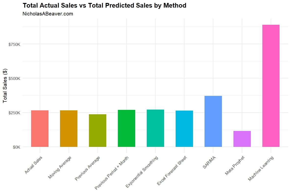
And the figure below shows the total sales predicted by each method for 2024 alongside the actual sales for 2024.

Diagnostics

As shown in the table and figures above, simpler methods did better overall. Let’s take a second look at that table:

As shown in the table above, Previous Averages, Previous Period + Month, and SARIMA had the best R-squared (though, admittedly, not spectacular).

The RMSE was similar for the simpler methods, and way off base for the latter three methods. sRMSE showed similar results, with SARIMA performing a little better here.

In terms of TAE, or “total absolute error”, Moving Average, Previous Period + Month, and Excel Forecast Sheet had TAEs < 1%. Exponential Smoothing fared decently here at 1.79%. The rest range from bad to simply ridiculous.

Considering only the diagnostics, the following table summarizes the best and worst methods:

Discussion

So what happened here?

In terms of diagnostics, Previous Period + Month knocked it out of park while Prophet and ML performed the worst.

How can this be?

For one, I’d like to again point out that this is a toy illustration of the points I wish to make here. For two, it is precisely the complexity of methods like Prophet and ML that made them fail.

Our dataset doesn’t contain the types of values we’d hope to have for either Prophet or the random forest ML model to work. And given our task, to simply forecast aggregate sales into a future period, more complexity simply isn’t necessary.

First, we must keep in mind that our knowledge about what already exists is limited. Even with increasingly large datasets, there are always more variables and more information outside our grasp than inside of it. This issue is compounded by the fact that if we accept the premise that the past is truly prologue to the future, or that with the right past information we can forecast future outcomes, the limit on the knowledge we wish we had today inherently hampers our ability to predict the future on that premise alone (to say nothing of further issues).

Second, we mustn’t confuse noise for signal. The Prophet and ML models, especially, try to interpret existing patterns and extrapolate meaning from them. In Prophet’s case it comes in the form of complex “changepoint” patterns. In ML’s case, its the interrelation of many covariates sampled randomly in order to discover some underlying pattern. But what if there is no pattern like those to be discovered? In that case: garbage in = garbage out.

Third and finally, we have to remember that complexity doesn’t equate to correctness. If we make fewer assumptions, and get a usable result, we should be happy with that result. Adding more complexity, more variables, more patterns, adds unneeded (and possible misleading and dangerous) beliefs into our models. The simpler methods abbreviate which variables contribute to the outcome we’re interested in to give us a rough idea that we can work with. The complex methods try to explain each and every change in many variables and how they contribute to some larger whole.

Conclusion

The point I wish to illustrate is that simpler is often better. Or at least, complexity doesn’t equate to accuracy or usefulness.

To better harness more complicated methods like Meta Prophet and the random forest machine learning method, we’d need different kinds of data. But given what we have, and perhaps given what our stakeholders are really asking for, even with such data at hand the results may not be desirable with these more complicated methods (nor would, perhaps, the exponentially larger amount of work required to use them).

The real issue, I think, is far beyond the scope of this one blog post, but I hope to explore in the near future: epistemology. What we can know, and whether we are certain that what we know is true, is limited. There are so many more variables outside of our model that we can never account for. In fact, I’d argue, that when we meddle in the real world by, say, introducing a sales promotion to boost sales on a product, we change the system we’re trying to measure and predict in, well, unpredictable ways.

The simple methods shown in this post—like our champion “Previous Period + Month”—abbreviate these many unknown variables for us. The ups and downs and wild swings in sales from month to month are easily mistaken as some kind of pattern. We’re prone to think that if we look at the data close enough, we’ll unlock the causal pattern that makes sales $X one month and $Y another month. This probably isn’t the case, because, once again our knowledge is limited and our very involvement in the system we’re trying to measure and predict is changing that system in real time before we realize what impact our meddling has caused.

Simple models are summarizing this for us. They deserve consideration, especially in light of our vast increases in available data and in light of our current obsession with all things artificial intelligence (AI). If smart human brains, as I believe, can’t figure the causal patterns out because they are either unknowable and/or our involvement changes them before we recognize it, no amount of “intelligence,” human or not, can know this either.

So what can we do?

I’d answer that with why I believe the “Previous Period + Month” model performed best in this exercise: it’s based on the simple logic of seasonality and momentum. Seasonality is a known and well documented phenomenon in sales: some months just see more sales than others due to a variety of factors. This is captured in our using the same month in the previous calendar year. Momentum is also a well known and well documented phenomenon: when you’re doing well, you tend to keep doing well, and when you’re doing poorly, you tend to keep doing poorly. I just combined these two and averaged them.

Simple as that.

I think a lot of analysts would chafe at such a suggestion. They would want more complexity. More variables. More precision. And I would agree with some of that, certainly.

But this simple method, based on simple, proven logic, works. Complexity didn’t help solve the problem. Logic did.