
Data and Problem Statement
Customer Service departments collect all kinds of data from customers. This data can be used to diagnose issues faced by customers, make them new offerings, and relevant to this project, gauge their satisfaction.
A Customer Feedback and Satisfaction dataset provided by Jahnavi Paliwal on Kaggle contains data for 38,444 customers. The dataset provides 11 variables, including the age, gender, country, income, and more for each customer. [1]
Key to this project is the variable SatisfactionScore, which is a continuous variable bounded to values on the interval [0, 100].
What we wish to know is: what regression model best fits predicting SatisfactionScore?
Which predictors should be used for the SatisfactionScore response? Which prior best suits this regression model? How accurate can we get?
Let’s find out.
Zero One Inflated (ZOI) Beta Model
The SatisfactionScore response in this model is densely distributed toward the upper tail. That is to say that a huge proportion of customer ratings are clustered at or near 100 (the top of the scale). This is a good thing for customer retention, but it creates a bit of a problem for modelling on commonly used distributions like the Gaussian (“normal”) distribution, among others.
Consider the distribution of SatisfactionScore from the data:
FIGURE 1. Distribution of SatisfactionScore Scores from the dataset.

That’s really skewed toward the top of the scale. A lot of customers are satisfied.
To model this, we’ll use a zero one inflation beta model. This model will allow us to set priors that define the probability of an observation’s value being either at 0 or at 1, and thus, influence the tailed-ness and values in between as they are pulled toward these extremes.
We’ll rescale our data down to fit on the [0, 1] interval required by the zero one inflation beta model, run our regression, then re-scale the values back to the [0, 100] interval.
BRMS Package in R
To accomplish this, we’ll be using the brms package in R. [2]
All of the R code used to run this model is available in the References section, below. [3]
Outline of Steps Taken
The R code used in this model [3] comes down to the following major steps:
- Import the dataset.
- Choose which predictors to select for the regression.
- Split the dataset into two parts: the “training” data (even-numbered rows) and the “validation” data (odd-numbered rows).
- Set priors for the zero one inflated beta model.
- Scale the data to the [0, 1] interval to suit the model.
- Run the model in brms.
- Check the summary, diagnostics, and plots of the model.
- Visualize the model’s performance against the actual observations.
Choosing Predictors
Figure 2, below, shows a scatterplot of SatisfactionScore against each of the other nine possible predictor variables. Only ProductQuality and ServiceQuality had reasonable correlations with SatisfactionScore (that is, correlation >0.5). However, when testing a mix of models using various combinations of predictors, the model presented here using Age, Income, ProductQuality, ServiceQuality, and PurchaseFrequency performed best.
The chosen predictors are shown in red in Figure 2, while those left unused are in black.
FIGURE 2. Correlations Between SatisfactionScore and the Nine Other Applicable Predictors.

Gender, Country, FeedbackScore, and LoyaltyLevel had no real bearing on predicting SatisfactionScore.
With these predictors in mind, we set ourselves to forming our model based on this basic outline:

Results and Inference
First, it must be said that several separate models were run and the best one, presented here, was used. The model selected had the right mix of relatively few predictors and high accuracy.
That aside, let’s first take a look at what our regression equation came out to be.
TABLE 1. brms Regression Output for the Selected Model.
Family: zero_one_inflated_beta
Links: mu = logit; phi = identity; zoi = identity; coi = identity
Formula: SatisfactionScore_scaled ~ Age + Income + ProductQuality + ServiceQuality + PurchaseFrequency
Data: data (Number of observations: 38444)
Draws: 4 chains, each with iter = 2000; warmup = 1000; thin = 1;
         total post-warmup draws = 4000

Regression Coefficients:
                  Estimate Est.Error l-95% CI u-95% CI Rhat Bulk_ESS Tail_ESS
Intercept             2.13      0.01     2.11     2.15 1.00     4131     3119
Age                   0.28      0.00     0.27     0.28 1.00     9288     2660
Income                0.42      0.00     0.41     0.42 1.00     9336     2780
ProductQuality.L      2.97      0.02     2.94     3.00 1.00     4430     2938
ProductQuality.Q     -0.07      0.01    -0.10    -0.04 1.00     5776     3224
ProductQuality.C     -0.06      0.01    -0.09    -0.04 1.00     6418     3053
ProductQualityE4      0.01      0.01    -0.02     0.04 1.00     6279     2867
ProductQualityE5      0.01      0.01    -0.02     0.03 1.00     5658     3096
ProductQualityE6     -0.00      0.01    -0.03     0.03 1.00     6973     2778
ProductQualityE7     -0.03      0.01    -0.06    -0.01 1.00     7101     2601
ProductQualityE8      0.02      0.01    -0.01     0.05 1.00     7497     3080
ProductQualityE9      0.00      0.01    -0.03     0.03 1.00     6385     2931
ServiceQuality.L      2.97      0.02     2.94     3.01 1.00     5264     3114
ServiceQuality.Q     -0.05      0.01    -0.08    -0.03 1.00     6062     3034
ServiceQuality.C     -0.05      0.01    -0.08    -0.02 1.00     7421     3147
ServiceQualityE4     -0.00      0.01    -0.03     0.03 1.00     7101     3089
ServiceQualityE5      0.00      0.01    -0.03     0.03 1.00     7011     3327
ServiceQualityE6      0.00      0.01    -0.03     0.03 1.00     6796     3319
ServiceQualityE7      0.01      0.01    -0.02     0.04 1.00     6158     3174
ServiceQualityE8      0.01      0.01    -0.02     0.04 1.00     6250     2720
ServiceQualityE9     -0.01      0.01    -0.04     0.01 1.00     5744     2909
PurchaseFrequency     0.03      0.00     0.03     0.03 1.00     4061     2918

Further Distributional Parameters:
    Estimate Est.Error l-95% CI u-95% CI Rhat Bulk_ESS Tail_ESS
phi     6.73      0.06     6.62     6.84 1.00     3398     3207
zoi     0.00      0.00     0.00     0.00 1.00     5131     2231
coi     0.89      0.10     0.64     1.00 1.00     4894     2288
So how does this model compare to the actual data?
FIGURE 3. Distribution of Actual (y) and Predicted (y_rep) Customer Satisfaction Scores.

Of note is the fact that our predictions (y_rep) tend to undershoot the actual values below about 90 and overshoot above about 90. Despite these limitations, however, after we re-scale the data we’ll see that this is a reasonable fit. In real life, we’d use this model as an initial trial and then continue to refine as new data became available.
At this point, we’ve regressed only on half the data: the training set.
Here are the actual Satisfaction Scores compared to our predictions only on the training set:
FIGURE 4. Actual vs. Predicted Satisfaction Scores using only the Training Dataset.

This round had an R-squared of:
    Estimate   Est.Error      Q2.5     Q97.5
R2 0.7785288 0.001954189 0.7745971 0.7823018
Not too shabby.
Next, we take the model, trained on the Training Dataset, and use it to predict the values of the validation dataset.
Here are the actual Satisfaction Scores compared to our predictions only on the validation set:
FIGURE 5. Actual vs. Predicted Satisfaction Scores: Model Trained on the “Training Set” and Used to Predict the Values of the “Validation Set”.

This round had an R-squared of 0.749671. We’re on to something here!
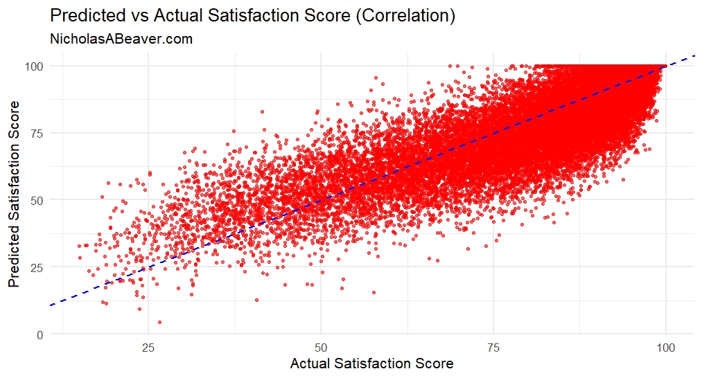
Lastly, the visualize the correlation of the actual values to the predicted values from the entire dataset:
FIGURE 6. Predicted vs. Actual Satisfaction Scores from the Entire Dataset.

The blue line is the the 1:1 correlation line (i.e., slope = 1). The dots represent where the actual SatisfactionScore aligns with our predicted SatisfactionScore. There is a very clear correlative trend and one that is supported by R-squared metrics of ~0.75 to ~0.78. A final check for the predictions made for the entire dataset reveals an R-squared of 0.7568339.
Conclusions
In this project, we’ve tried to predict SatisfactionScore from a dataset of over 38,000 customer observations. We found a good mix of predictors from the data to make these predictions.
Our resulting model is a zero one inflation beta model, which allows us to skew our data very heavily toward the upper bound of the scale. This model allows us to more accurately predict the actual SatisfactionScore values which are heavily clustered around this upper bound.
Our model provided us with adequate accuracy (R-squared of ~0.76), without too much risk of overfitting (since we relied on about half of the available predictors, cutting out some of the noise that could be introduced to the model should we have used them all).
Further Work
Some further work can be done using this model. These may be the subjects of future projects on this website:
- How could this model be used as a prior for a new Bayesian update with new data? What inferences could we draw after performing this update?
- What are the causal effects of the predictors on CustomerSatisfaction? For instance, what would these scores be if every customer purchased 1 more product? Or what would they be if our average customer base was 10 years older? This would require counterfactual models.
- What are the casual factors leading to low CustomerSatisfaction? Why are these customers so unhappy? What inferences could be drawn in this regard from the available data?
References
- Paliwal, J. (n.d.). Customer Feedback and Satisfaction [.csv file]. https://www.kaggle.com/datasets/jahnavipaliwal/customer-feedback-and-satisfaction
- Bürkner, P.C. (2017). brms: An R package for Bayesian multilevel models using Stan. Journal of Statistical Software, 80(1), 1–28. https://doi.org/10.18637/jss.v080.i01
- Beaver, N. (2025). Predicting Customer Satisfaction Scores with Zero One Inflated Beta Model [R code]. Published 28 June 2025. https://www.nicholasabeaver.com/wp-content/uploads/2025/06/predicting_customer_satisfaction_scores_with_zero_one_inflated_beta_model_r_code.txt