Rent vs. Purchase of a Home: Projection Over 31 Years (with Excel Modeling Tool)

Housing affordability is a major concern among Americans today.

According to the National Association of Realtors, the median age of a first-time homebuyer has risen to an unprecedented 40 years old and the share of first-time homebuyers has contracted by 50% since 2007. [1]

This sobering reality leaves us with some open questions: Does it make sense to buy? If one does buy, should it be a 30 or 15-year mortgage? What outcomes could be expected for buying or renting?

This project aims to help answer those questions by providing an Excel Tool (linked below) that allows the user to input relevant financial assumptions and model renting vs. buying scenario outcomes over several decades. This project post demonstrates the use of that Tool.

What This Project and the Excel Tool Aim to Do

This project envisions three parallel universes:

The individual or family purchases a home with a 30-year fixed rate mortgage
The individual or family purchases a home with a 15-year fixed rate mortgage
The individual or family rents a home

These three universes run side-by-side based on assumptions we make on the purchase price, down payment, interest, etc. (more on those below).

We assume that the individual or family can afford all three scenarios, and thus will have the same amount of money available each month.

In each of these three scenarios, the individual or family invests anything not spend on housing expenses into an investment portfolio (outlined below in our assumptions). This continues for 31 years.

At the end of the simulation we analyze the financial outcomes and draw conclusions about the drivers of these results.

This analysis seeks to illuminate the potential financial trade-offs between renting or owning a home and provides a tool to use to make such analysis individualized for one’s own circumstances.

The Excel Tool & a Word About Individual Circumstances

The Excel Tool developed and used for this project is available here. (We link to it again in a later section.)

The Tool allows the user to input his or her own financial assumptions and create different projections based on different circumstances.

All of the results are directly based on the financial assumptions used. For this demonstration, we use a real life example home and its attendant figures (the home selected is discussed below in a later section).

That being said, individual circumstances vary.

Home or rent prices, interest rates, assumptions for down payments, repairs, maintenance, and taxes, etc. can and will be different for different people at different times and different places.

Nothing in this demonstration should be construed to mean that these assumptions or results are definitive.

Your mileage may vary.

Why 31 Years?

We choose a simulation period of 31 years to give a more fair comparison between the three universes.

If the simulation were shorter, the outcomes would be very different for a homebuyer with a 30-year mortgage with little exposure to stocks and bonds, a homebuyer with a 15-year mortgage and a lot more exposure to stocks and bonds, and a renter will full exposure to stocks and bonds.

We give our models another year after the repayment of the longer mortgage to allow each investment (a home and/or investment portfolio) more time to compound. This allows the long-term potential of each investment to become more apparent.

The Excel Tool allows the user to see results for any year of the simulation (from Year 0 to Year 45) by changing a selector on the Results tab.

The House

This demonstration of the Excel Tool uses a single house currently for sale in Richardson, Texas [2]:

We use the figures presented in this listings for the assumptions outlined in the section below.

The homebuyers (either 30-year or 15-year mortgage) will purchase the home for $425,000 in their scenarios while the renter will rent the same home for an initial monthly rent of $2,756 per month (as explained below).

Thus, all three scenarios will buy or rent the exact same property.

Financial Assumptions Used in this Project

Using the Excel Tool, we make our key assumptions, which are explained below:

1. Purchase Price

The purchase price of the listed home is $425,000. [2]

2. Down Payment

We assume a 20% down payment on the purchase price: $85,000.

3. Closing Costs

Using Fannie Mae’s closing costs calculator for the home price in Dallas County, TX, we find that “middle” estimate closing costs are $15,384. [3]

From this we subtract the $500 listed by the Fannie Mae calculator for Homeowners Association (HOA) Dues (since the listed house does not reside in an HOA area) to arrive at closing costs of $14,884.

4. Agent Commission

According to Realtor.com, real estate agent commissions can range from 5 to 6% of the home’s sale price. [4] Rates can be negotiated and are nowadays paid by both the buyer and seller.

For our assumptions, we take the midpoint of the Realtor.com estimate (i.e., 5.5%), split evenly between the buyer and seller. This leaves us with a computed commission due by the buyer of $11,688.

5. Interest Rate and Mortgage Payments

As of the end of Q2 of 2025, the Federal Reserve reported an average interest rate of 6.72% for a 30-year fixed rate mortgage [5] and an average interest rate of 5.85% for a 15-year fixed rate mortgage [6].

This leads to monthly mortgage payments of $2,198 and $2,842, respectively.

We assume all mortgages for this project to be fixed rate.

6. Private Mortgage Insurance (PMI)

Private Mortgage Insurance (PMI) is not included in these models, as our down payment is 20% or more.

If the Excel tool is filled in with a down payment that is less than 20% of the purchase price, PMI will automatically be applied to the homeowner models based on the rate that is inputted (suggested 0.5 to 1.5%).

7. Initial Rent Price

Zillow includes an estimated monthly rental price of $2,756 for the property. [2]

We assume this as our initial monthly rent.

8. Security Deposit and Insurance

The rental security deposit is set as equal to the initial rent price ($2,756).

This amount is deducted from the amount of funds available to invest at the start of the modeled period and is kept on balance as a prepaid expense (thus, is added to the renter’s net worth going forward as it would theoretically be paid back after the rental property is vacated).

A security deposit is an unproductive asset on the renter’s balance sheet (and a liability on the landlord’s).

9. Renters Insurance

Bankrate reports the average renters insurance in the United States as $14 per month. [7]

For reasons listed below in the Homeowners Insurance section (i.e., Texas’ homeowners insurance costs are 61% above the national average), we list the renters insurance in the Assumptions as $23.

The model assumes payments for insurance are set aside monthly.

10. Repairs & Maintenance

State Farm advises an annual repairs and maintenance budget of 1 to 4% of the home’s value. [8]

We take the midpoint between these estimates: 2.5%.

The model assumes payments for these payments are set aside monthly.

11. Property Tax

For 2025, the home listing had an assessed value of $415,940 with an annual property tax due of $4,032. [2]

This equates to an approximately 1% annual property tax rate.

The model assumes payments for these taxes are set aside monthly.

12. Homeowners Insurance

Bankrate reports the average Texas insurance as $3,899 per annum. [9]

This is approximately 61% above the reported national average of $2,424.

The model assumes payments for these payments are set aside monthly.

13. Homeowners Association (HOA) Fees

The listing for sale does not have HOA fees. [2]

14. Portfolio Return & Dividend Rate

The investment portfolio chosen for this model is based on the Vanguard Total Stock Market Index Fund Admiral Shares (ticker: VTSAX). [10] The fund has a $3,000 minimum investment, which isn’t an issue for the Renter model; in the case of either Homeowner model, the equivalent Exchange Traded Fund (ETF) can be used in its stead. [11]

Based on the performance of VTSAX since its inception (in November of 2000), our assumed portfolio will have an annual pre-tax portfolio return of 8.88% and an annual pre-tax dividend of 1.08%.

(Note that the dividend is part of the compounded return of 8.88%; we break out the dividend assumption to help compute income taxes due on the fund’s distributions).

15. Income Tax Rate

We assume a 15% income tax, which is the rate paid by most investors (i.e., currently, 15% is paid on annual dividends between $47,026 and $518,900). [12] To keep things simple, we do not assume the lower 0% bracket (currently for annual dividends below $47,026). This will slightly favor the homeowner models, but isn’t enough to disrupt the final results meaningfully.

This is the federal rate only: Texas has no state income tax.

This income tax applies only to the dividends paid by the portfolio.

The model assumes payments for income taxes are set aside monthly.

16. Investment Fees

VTSAX has an annual fee of 0.04% of assets under management.

The model assumes payments for these fees are set aside monthly.

17. Home Value Increase

The Federal Reserve reports an all-transactions House Price Index which saw increases from 59.99 in 1971 to 706.04 in Q2 (July 1) 2025 [13].

This leads to an average home price increase of 5% per annum (or ~0.41% monthly).

18. Rent Price Increase

The Federal Reserve reports the Consumer Price Index of rents having increased from 84.7 to 436.152 from January 1981 through Q2 (July 1) of 2025 [14].

This leads to an average rent increase of 3.74% per annum (or ~0.31% monthly).

A Few Other Assumptions

Additionally, some additional implicit assumptions are made for the sake of simplicity and clarity:

Homeowners do not rent space in their own homes or otherwise collect income from owning the property.
Homeowners will not refinance their homes.
No shares in the portfolio are sold, ever. Investors buy and hold the portfolio and pay taxes and fees as applicable.
The assumption figures are set and applied continuously throughout the model.
Each model has the same amount of money available each month. Anything not spent on housing expenses is invested in the portfolio.

Models

We use our assumptions in three models: 30-Year Mortgage, 15-Year Mortgage, and Renter.

These models assume three possible universes in which the same individual or family is making the decision to put available resources into a 30-year mortgage, 15-year mortgage, or to rent a home.

The reader should keep in mind that all three models are buying or renting the exact same house.

Our models perform as follows:

All three models are assumed to have the same amount of money to invest each month for 31 years. This amount is based on the maximum payments from any of the three models. Thus, all three models have the same funds available to divvy up.
Each model pays mortgage, rent, and other expenses (repairs and maintenance, property taxes, insurance). Anything that’s left is invested in the portfolio, which is subject to income tax and fees. These figures are computed monthly.
At the end of 31 years (or 372 months), we compare the outcomes.

Results & Analysis

After 31 years, we analyze the results of our simulation based on our assumptions.

Comparison of Ending Net Worth by Model

Of the three models, the renter comes out far ahead of the two homeowning models as shown on the Table 1 below:

The renter comes out approximately $488,000 ahead of the average of the two homeowner models.

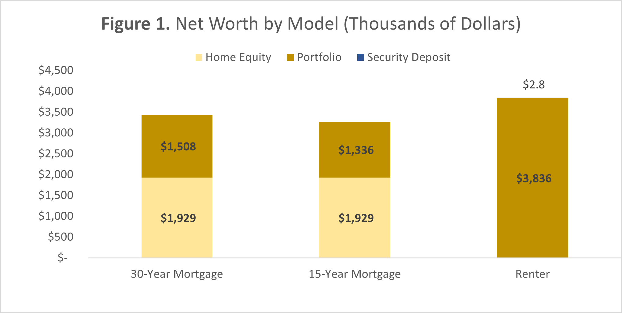
The composition of each model’s net worth at the end of the simulated period is visualized below in Figure 1:

The net worth by model over the 31-year simulation is illustrated in Figure 2:

Internal Rates of Return (IRR) by Model

The Internal Rates of Return (IRR) for each model are illustrated in Figure 3:

Figure 4 shows the change in IRR over the 31-year simulated period

As measured by IRR, the homeowner models come out ahead of the renter. The renter’s IRR is what we would expect from pure exposure to the investment portfolio’s return (minus fees and taxes) and the cost of renters insurance.

It should be noted that the IRR for the homeowner models changed markedly over the simulated period as the home in either scenario is paid down. The renter’s IRR remained consistent.

The higher IRR for both homeowner models is explained by the more efficient use of leverage to paydown the mortgage while simultaneously experiencing increases in the equity of the home. The homeowner models also benefited from the imputed savings from rent (i.e., in each month, the IRR figure for each homeowner model was adjusted to reflect the savings of not paying rent). In other words, these models had added to their net cashflows for IRR computation the amount of rent paid by the renter).

Despite the higher IRR for the homeowning models, the ending values for either of them still came out behind the renter.

Total Return by Model

By “total return” we mean simply the net difference between assets owned by each model and all payments made by each model.

Again, the renter comes out far ahead, as shown on the Table 2, below:

(Note: Total payments, above on Table 2, vary slightly from model to model due to the effect of income taxes and investment fees which were paid from the monthly net asset value (NAV) of the investment portfolio.)

The renter had a total return of $1.24 million. The renter’s total return was 47.9% on its total payments of $2.6 million.

Conversely, the homeowners had a $824,873 and $704,870 total return, respectively. The corresponding total return rates were markedly lower than the renter’s.

While all three models had roughly the same amount of payments (about $2.6 million) over the simulated period, the renter’s assets were worth more. The renter’s use of capital was more efficient.

The total return in dollars and as a percentage of total payments made is illustrated below in Figure 5.

Annual Dividends and Expenses

Lastly, we look at the dividends paid out by each model’s investment portfolio and compare them to each model’s housing expenses.

By Year 31, the renter is able to cover 37.3% of his or her housing expenses from after-tax dividends alone. The homeowner models are not so fortunate.

Because the renter has a much larger investment portfolio, he or she is able to cover much more of his or her housing expenses through his or her dividend payments. This is despite the renter’s living expenses and income tax being higher than either homeowner model.

Figure 5, below, shows the comparison visually for each model:

Downloadable Excel Tool

The Excel modeling tool used to conduct this analysis and generate the tables and figures shown in this post can be found below:

Rent vs. Purchase of a Home: Projection Over 45 Years (Excel Tool)

You are encouraged to plug in your own assumptions and see what outcomes are possible.

Conclusion

The results may come as a shock to some.

The accepted wisdom in the United States has seemed to be that purchasing a home is the only way to avoid flushing money down the proverbial toilet.

The three models result in similar outcomes. While it’s true that the renter ends up with about $488,000 more than the average of the homebuyer models, this equates to a real difference of about $195,000 in 31 years (assuming a 3% inflation rate).

While the financial outcomes are all fairly similar, let’s look at the position of each.

Asset Mix

The homeowners each end up with a house valued at $1.9 million and portfolios of $1.5 and $1.3 (for the 30-year mortgage and 15-year mortgage respectively).

The renter ends up with a $3.8 million portfolio (and a security deposit on the books for $2,756).

We might assume that the 15-year mortgage model would have a larger investment portfolio due to having paid off the home sooner; but the opposite is true.

This is explained by the next point.

Leverage

The homeowners put leverage (i.e., borrowed money) to work. Because of this, their mortgage payments were fixed while the value of the home was simultaneously increasing. This led to larger IRR’s for both homeowner models.

The renter did not have an advantage from leverage.

But why, despite the homeowners eventually having no mortgage to pay and the renter’s monthly rent increasing every year did the renter come out (a little) ahead?

Investment Productivity

The homeowners, even after considering principal and interest payments on their mortgages, still had to pay over 3.5% per annum (for repairs, maintenance, and property tax), indefinitely, to maintain their homes. The costs of repairs and maintenance, property tax, and insurance mounted. These payments supported the 5% per annum value increase of the home. Neglecting to maintain the home can lead to lower valuations. Ugly, unkept houses, or those that are falling part from lack of care, are worth less than well-maintained homes.

Despite the advantage of leverage, homeowners are spending 3.5% of the home’s value each year to see gains of 5%.

Even though the renter’s rent increases, the growth of the investment portfolio is far higher (8.72% per annum after taxes). And the fees for maintaining it are very low (0.04%). Thus, the renter can not only keep pace, but slightly outrun the homeowners.

It’s important to note that the renter had a large head start from the outset of the simulation: while the homeowner models sunk $111,572 each in cash to close, the renter put this money to work (minus the security deposit) right away in the investment portfolio. All those years of compounding, and all those years of new investments, made all the difference.

This is also why the 30-year mortgage model beat out the 15-year mortgage model: the 30-year model had more money sooner to set aside for the investment portfolio. While the 15-year model was busy paying off the loan at an accelerated rate (all to gain 5% per annum), the 30-year model paid off the loan more slowly but had more and longer participation in the investment portfolio’s 8.88% per annum growth.

Parting Thoughts

The conclusion is ultimately about the use of capital: a homeowner uses available capital to maintain his or her dwelling’s value while a renter puts the same available capital into a productive asset.

All of this is to say nothing, of course, about preferences. It is perfectly reasonable to wish to own and occupy one’s own home. There is the pride of ownership, tranquility, and space to consider. A homeowner can do what he or she likes with the home, while a renter cannot.

But given the home over several decades, a renter who spends what a homeowner does on rent and a widely-diversified investment portfolio wins the financial race, all while maintaining the flexibility and convenience of being a renter. (If the dishwasher breaks, or the toilet overflows… call the landlord.)

The financial results, however, are remarkably close to one another despite such drastic differences in asset mix between the two homeowner models and the renter model. This shouldn’t come as a surprise, either: the market for capital is overall an efficient one. Landlords, renters, homebuyers, and stock investors all have access to the same choices. Capital moves to where it is most productive, evening out the long term returns for the three models.

(However, check out what happens beyond Year 31. Productivity is magnified!)

All this is given the assumptions we’ve modeled. The reader is encouraged to use the Excel Tool to model other scenarios.

References

- NAR (2025). First-Time Home Buyer Share Falls to Historic Low of 21%, Median Age Rises to 40. National Association of Realtors. Published 4 November 2025. Accessed 15 December 2025. https://www.nar.realtor/newsroom/first-time-home-buyer-share-falls-to-historic-low-of-21-median-age-rises-to-40
- Zillow (2025). 431 Malden Dr, Richardson, TX 75080 [Home Listing]. Zillow.com. Updated 6 December 2025. Accessed 15 December 2025. https://www.zillow.com/homedetails/431-Malden-Dr-Richardson-TX-75080/27167547_zpid/
- FNMA (n.d.). Closing Costs Calculator. Fannie Mae (Federal National Mortgage Association). Accessed 15 December 2025. https://yourhome.fanniemae.com/calculators-tools/closing-costs-calculator
- Buch, Clarissa (2025). Who Pays the Real Estate Commission and Closing Costs: The Homebuyer or Seller? Realator.com. Published 3 November 2025. Accessed 17 December 2025. https://www.realtor.com/advice/finance/realtor-fees-closing-costs/
- FRED (2025). 30-Year Fixed Rate Mortgage Average in the United States (MORTGAGE30US). Federal Reserve Bank of St. Louis. Last updated 26 November 2025. Accessed 3 December 2025. https://fred.stlouisfed.org/series/MORTGAGE30US
- FRED (2025). 15-Year Fixed Rate Mortgage Average in the United States (MORTGAGE15US). Federal Reserve Bank of St. Louis. Last updated 26 November 2025. Accessed 3 December 2025. https://fred.stlouisfed.org/series/MORTGAGE15US
- Cox-Steib, J. (2025). Average cost of renters insurance in 2025. Bankrate.com. Updated 1 November 2025. Accessed 15 December 2025. https://www.bankrate.com/insurance/homeowners-insurance/renters-insurance-cost/
- State Farm (2025). How much to budget for home maintenance. Published 13 November 2024. Accessed 15 December 2025. https://www.statefarm.com/simple-insights/residence/how-to-budget-and-save-for-home-maintenance
- Todroff, N. (2025). Average homeowners insurance cost in December 2025. Bankrate.com. Updated 1 November 2025. Accessed 15 December 2025. https://www.bankrate.com/insurance/homeowners-insurance/homeowners-insurance-cost/#cost-by-state
- Vanguard (2025). Vanguard Total Stock Market Index Fund Admiral Shares (VTSAX). Vanguard.com. Updated 30 November 2025. Accessed 15 December 2025. https://investor.vanguard.com/investment-products/mutual-funds/profile/vtsax
- Vanguard (2025). Vanguard Total Stock Market ETF (VTI). Vanguard.com. Updated 30 November 2025. Accessed 15 December 2025. https://investor.vanguard.com/investment-products/etfs/profile/vti
- Vanguard (n.d.). Taxes on dividend income. Vanguard.com. Accessed 15 December 2025. https://investor.vanguard.com/investor-resources-education/taxes/dividends
- FRED (2025). All-Transactions House Price Index for the United States (USSTHPI). Last updated 25 November 2025. Accessed 15 December 2025. https://fred.stlouisfed.org/series/USSTHPI
- FRED (2025). Consumer Price Index for All Urban Consumers: Rent of Primary Residence in U.S. City Average (CUSR0000SEHA). Last Updated 24 October 2025. Accessed 15 December 2025. https://fred.stlouisfed.org/series/CUSR0000SEHA